Follow the first link above for the latest version of MOPlot

MOPlot

program for Plotting Molecular Orbitals (and other stuff)
version 1.8x for Windows 2000/XP, Linux, and Mac OS9/X

Contents

Introduction and a bit of history

Although many programs are available that can produce very pretty and quantitatively accurate electron density plots from the outputs of quantum chemical calculations, the computation of each such plot is rather time-consuming, even on current hardware, so viewing several molecular orbitals, e.g. to choose a set to include in an active space, may require a considerable degree of patience.

In addition, the resulting images often do not immediately reveal the "nature" of a molecular orbital very clearly, and images must be turned and twisted around before one gains insight, e.g. into the nodal structure (note that people who use such plots in publications usually have to display several views to make them intelligible to the readers).

In our work we felt the need for a program that would allow us to flip rapidly through a set of MOs, such as to have an immediate view of their nodal structure and an approximate idea of their spatial distribution over a molecule. The graphic tools implemented in GaussView, Spartan, CaChe, Hyperchem etc. visualize MO's as three-dimensional electron density plots which take some time to calculate and do not always readily yield insight into the nodal structure of MO's. Also, we were tired of trying to adapt the voluminous pixel images produced by the above electron density display programs for use in publications, so we wanted a utility that produces vector output.

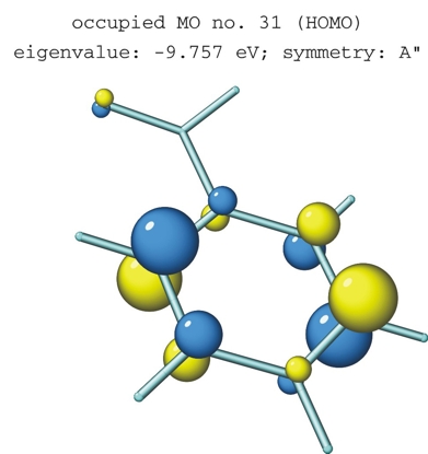
HOMO of admantylidene displayed by
GaussView (left) and MOPLOT (right)

MOPLOT fills this gap by producing 2-D projected images of geometries, MO's and normal vibrations produced immediately from the output of various standard quantum chemical programs.

An solution that fulfils all of the above requirements had actually been proposed and implemented on a PDP 8 computer over 30 years ago by Haselbach and Schmelzer with the purpose of displaying MOs from semiempirical calculations in the ZDO approximation. In the 1980s we adapted a copy of this Fortran program to PCs running DOS, and later to the Windows operating system. Since the 1990s we used it also to display MOs from ab initio calculations, although we had to cut some corners to do that (see below).

However, the advent of Windows NT/2000 (which lacks a DOS kernel), tolled the death bell to MOPlot, so it began to fall into disuse, and students went back to make guesses about the shapes of orbitals instead of viewing them.

Then we had the good fortune to gain the collaboration of Dr. Rouslan Olkhov who, while waiting for parts for a laser system to arrive, agreed to look into the MOPlot problem. After thinking about this for a moment, Rouslan proposed to rewrite MOPlot from scratch, using the LabView programming environment. At first we were a bit incredulous, but it was not long before Rouslan produced the first MOPlot-style pictures of MOs that looked much prettier than anything we had had before. In addition it turned out that the user interface was much easier to program than with any version of Fortran, so we decided to scrap all the code we had and build on what Rouslan was producing.

After about six months, he had the first full working version of MOPlot, and ever since he has been ironing out bugs, adding features (see below), and refining the user interface until he arrived at the present version which is not only much better than anything we had before, but has the advantage that it runs on any platform and operating system for which LabView exists, i.e. Windows, Linux, MacOS. As our University holds a site licence to the LabView professional development system this makes it possible for us to offer compiled versions of MOPlot for all these platforms which run independently of the LabView programming environment.

Overview of MOPlot program

MOPlot can display

• geometries, including the Cartesian coordinate axes, atom numbers according to the geometry definition in the calculation. Molecules can be turned in all directions under mouse control, or, for more precision, using the controls in the "camera" menu. Bonds can be displayed as cylinders or as simple lines.
• Mulliken atomic charges, group charges (charges of hydrogens summed into heavy atoms), and atomic spin populations (for open shell systems), if the corresponding information is available in the output of the calculation.
• molecular orbitals (hence the name of the program), according to the protocol defined by Haselbach and Schmelzer and described below. MO's can be from RHF; UHF alpha/beta (cf switch in the "MO" menu), or CASSCF calculations. SCF MOs are ordered by energies, CASSCF MOs or natural orbitals are ordered by occupation numbers.
• normal vibrations, both as displacement vectors and in animated form. For complex molecules where the calculation of the displacements may become slow, a "loop" mode is available to speed up the animation.
• the gradient difference and derivative coupling vectors at conical intersections, as well as any linear combination of the orthonormalized vectors.

In addition, MOplot can

• compute geometric parameters (bond lengths, angles, dihedrals) for any set of atoms or midpoints between two atoms (the latter is a unique feature of MOPlot).
• plot the energy change in the course of a geometry optimization or a "scan" run (similar to Molden). The geometry at each step of the optimization can be displayed and saved to a file.
• form linear combinations of vibrations. This feature is useful for example to visualize the circular movement of atoms along degenerate normal modes (presently the different frequencies of non-degenerate modes are not taken into account).
• generate (interpreted or encapsulated) postscript output in vector format, using a flat or a pseude-3D shaded mode. Pages can be configured to hold multiple images of any kind that can be displayed on the screen. MOPlot output can thus be imported into most current drawing programs (Adobe Illustrator, CorelDraw …) for further processing.
• recognize output from Gaussian 94/98/03 calculations, and input to the Molden viewing utility, such as it is for example generated by the Molcas program. In addition, we have defined a proprietary standard format which MOPlot also recognizes. Specifications for that format can be found on the MOPlot webpage. Users who want to interface MOPlot to their favorite quantum chemical program should write scripts that convert the output of that program into the standard format. A sample Fortran program to achieve this is also provided on the MOPlot webpage.
• be freely configured by the user with regard to colors and fonts that appear in the various displays. In addition, a toggle is available to switch between color and b/w renditions, e.g. for publication purposes

MOPlot has a help mode where all the features in the different menus are explained in pop-up windows when one moves with the mouse over the feature on which one would like to get information.

Rules for drawing MO's
[Haselbach and Schmelzer, Helv. Chim. Acta 54, 1299 (1971)]

An LCAO-representation of MO's is given in the ZDO approximation (no overlap densities). AO contributions are

displayed as single spheres (pure s-AO's), or pairs of contiguous spheres (pure p-AO's) whose (combined) area is proportional to the contribution of an AO to the electron density at the atom on which this AO is centered

In s/p hybrid MO's, the area of one sphere is enlarged relative to the other in proportion to the size and sign of the s-contribution. If c(s)>c(p), a single sphere is drawn whose center is displaced in the direction of the (px, py, pz) vector in proportion to the p-contribution. (in MOPlot, the s/p ratio threshold where the display switches from pairs of spheres to single spheres can be changed. The default value is 1)

An illustration of this on a progressively pyramidalized methyl radical is shown below:

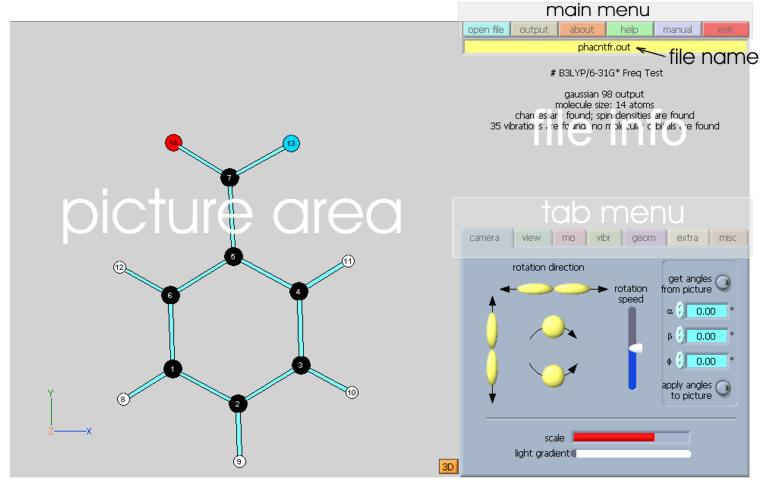
Limitations and caveats

It is important to remember that MOPlot was originally developed for viewing the results of semiempirical calculations to which the ZDO approximation is inherent. Its MO display mode reflects these theoretical models and MOPlot should therefore not be regarded as a program that yields accurate renditions of ab-initio wavefunctions. If this is what one wants, one should resort to one of the many fancy commercial or shareware electron density plotting packages (e.g. Spartan, GaussView, Molekel ...) which do an admirable job at that. The main purpose of MOPlot is to gain quick insight into the nodal properties of MOs and their approximate distribution over a molecule. These features can be more easily recognized in a ZDO-type rendition, such as it is provided by MOPlot.

MOPlot knows only about AO-coefficients, it ignores that fact that the same AOs have different exponents in different atoms. As long as one stays in the CHON group of atoms and within the realm of valence MOs, the errors introduced by this are usually quite tolerable and certainly not misleading, but if one does e.g. hydrogen fluoride, the results have very little relation to reality with regard to the electron density distribution. Also, to keep things simple, the contributions of inner and outer split valence basis AO's are simply summed up and polarization functions are ignored. After this, MOs are renormalized to one, ignoring overlap, to make them comparable amongst each other.

MOPLOT is not a commercial piece of software, and we can assume no responsibility whatsoever with regard to its performance. We have tested it to the extent that we can, and it looks as though it runs quite reliable. Nevertheless users are very likely to encounter bugs here and there and we would be very indebted if users would take the time to communicate these bugs to us.

MOPlot program interface

When you first open the program you are presented with a stark gray square on the left hand side of the program window (the picture area), and with a collection of menus on the right hand side. Before you can do anything, you must read a file by clicking on the blue "open file" button whereupon you are presented with a standard file selection window. MOPlot can only open Gaussian outputs, Molden inputs, and files in its proprietary standard format. If you try for example to open a Word document, MOPlot will complain.

Gaussian outputs can assume gargantuan sizes. Since MOPlot must plough through the entire output until it can be sure that is has found everything it needs, opening a file can take a little while. Don't despair, eventually it will get there, and it will display in the area below the menu bar what it found.

Once a file has been successfully read, the screen should look something like this:

The buttons in the menu bar allows the user to [open (a new) file], to prepare postscript [output] of pictures observed in picture area (see instructions below), to get some information [about] the authors of the program, and, finally, to [exit] the program and free the precious memory of the user’s computer.

The picture area is simply the graphics display and has no active interface elements., apart from the fact that you can twist and turn the molecule in all (hopefully intuitive) directions by dragging the mouse over it while you hold down the(left) mouse button. Pressing the shift key while you drag the mouse allows you to rotate the molcule in the plane of the display. Note the little coordinate system on the left bottom: it indicates the axes with regard to which the cartesians of the molecule were defined in the output.

The tab menu contains all the control elements, which allow user to manipulate the data to be shown in the picture area. Six pages are accessible in the tab menu:

[camera] is provided for more precise control over the rotation of the molecule around three perpendicular axes. A slide allows an adjustment of the [rotation speed]. At any moment the set of Eulerian angles, which correspond to the current orientation of the molecule in the picture area, can be memorized via [get angles from picture] into the a, b and f fields. The [apply angles to picture] button allows to instantly change the orientation according to the rotational angles entered in the a, b, and f fields (this feature can be used to re-establish a particular orientation). Finally there is a [scale] slide to increase or decrease the size of the molecule, a [light gradient] slide, which adjusts the depth hue, and [3D shading] button to invoke pseudo-3D rendering of the picture.

Note that the shaded spheres look much nicer in the postscript output than they look on the screen where the number of hues is kept small to maintain the quickness that is the prime quality of MOPlot.

[view] allows to select what one wants to view (except for MOs and vibrations, those are controlled in their own menus). Atoms are represented as circles whose radii are proportional (including the factors from the scale slides) to:

[atomic size] - approximate van der Waals radius of the atoms;
[atomic charges] - Mulliken atomic charges;
[group charges] - atomic charges with hydrogens summed into heavy atoms;
[spin population] - Mulliken atomic spin populations.

• By default atoms are colored according to their nature following to the usual conventions (H: white, C: black, N: blue, O: red, halogens: green, etc.). If one does not like this, one can toggle to [monochrome] according to the colour list in the [misc] menu. [labels] permits to mark the atoms with their ordinal numbers [type], or by their number in the input geometry [no.].
• Atomic sizes, charges, spins, and the bond thickness can be scaled using the corresponding slides at the bottom of the menu.
• If some bonds are missing or one wants to add a special bond, for instance a hydrogen bond, the two text fields, [normal] and [dashed], are provided, where extra bonds can be requested by entering pairs of atom numbers separated by single space, one pair per row. To update the picture with the extra bonds press the [extra bonds] button. Although "dashed" bonds appear thin but solid on the screen, they are dashed in the postscript output pictures.
• The [Add dummy] button creates a dummy atom between a pair of existing atoms, which are specified in two input fields below (such dummies may for example serve to draw bonds in metalloorganic complexes).

Note however that, once created, dummies cannot be removed! But, of course, one can always reload the original file.

[mo] controls the display of MOs:

• [show MO] must be activated to display MOs; the first MO that is displayed is the HOMO. Any other MO is chosen by its [orbital number]. One can always return to the [HOMO] or the [LUMO] by clicking the corresponding buttons.
• [alpha] [beta] toggle between alpha and beta MOs that make up an unrestricted wavefunction;
• [MO scale] scale the size of the MOs (without changing the molecule's size).
• [reverse phase] reverse the phases of the displayed MO (this is sometimes useful if one needs to correlate MOs of two species).
• [s/p ratio threshold] slide controls the s/p ratio at which the display switches from pairs of spheres to single spheres (see the above "Rules for drawing MOs")
• [add range of MOs] is only active when output is being prepared. It allows to add a range of MOs to the current page displaying them individually in the picture area during the process.

[vibr] controls the display of normal modes (vibrations)

• [show vibration] must be activated to display normal modes. The mode with the lowest (ev. the most negative) frequency is displayed. Any other modes may be chosen by their [number].
• [vectors] default display mode. Arrows are added to each atom which extend from them along the directions of a normal mode. Note: dummies carry vectors!
• [3D shape] vectors are represented not by traditional arrows but rather by two-color spheres: radii correspond to the amplitude and color distribution to the direction of the vibrational motion:



 

"spherical vectors" after: W. Hug, Visualizing Raman and Raman optical activity generation in polyatomic molecules. Chemical Physics (2001), 264(1), pp. 53-69



• [animation] animate the vibration currently displayed. The [amplitude] and the [animation speed] can be adjusted with the slides below. For large molecules the animation speed is limited by the capabilities of the processor. If one finds the animation too slow one can switch to
• [loop animation] which simply loops through a series of pictures without performing any computation.

 

Note: one has to leave the loop mode before doing anything else.

 

• [save coordinates] save a set of coordinates that correspond to a displacement of the atoms from their equilibrium positions along the normal mode currently displayed, scaled by [amplitude scale]. This has proven very useful e.g. in finding transition states starting from second order saddle points.
• [mix] mix the currently displayed mode with that selected in the box at the bottom. This works only in [animation] mode. The dial to the right allows to chose the phase with which the two modes are mixed (0˚ - in phase / 90˚ - out of phase). This option was designed in particular to visualize the circular motions that atoms undergo when they "vibrate" in degenerate normal modes. To show this, chose a set of two degenerate modes and a phase of 45˚.

Note: If the frequencies of mixed vibrations are different, the program treats them as if the ratio of their frequencies were integer from 1 to 6 (six is a maximum since the cartoon is limited by 20 frames and we need at least 3 frames per vibrational period).

[geom] is a utility to calculate geomety parameters (bondlengths and –angles, dihedrals) between 1-4 points in the molecule that is currently displayed. The unique feature of MOPlot is, that these points may but need not coincide with atoms, they can also be midpoints between atoms (in which case, instead of a single number, the input to the boxes on the right consists of two numbers separated by a "-"). This has often proven to be very useful to calculate, e.g. the angle between the two benzene rings in 9,10 dihydroanthracene.

When entering numbers, one may toggle to the next field with Tab. However, after entering the last number, one must click with the mouse somewhere outside the boxes to activate the calculation (just hitting "Enter" at the end will not do!)

[List feasible bonds] button creates a list of atoms that appear to be linked by chemical bonds along with bond lengths. This list can be saved to an ASCII file or copied into the clipboard.

[extra] The first extra feature is the option to view the course of geometry optimisations, similar to Molden. Initially an autoscaled plot of all the steps is displayed, with the relative energy set to zero for the first point.

With the magnifying glass one can zoom in on different parts of this plot with various options (or undo a zoom operation). With the hand one can move the plot around, and with the cursor tool one can grab the cursor and place it on any desired point (initially it is on the last point which is where one has to fetch it first), whereupon the geometry of this point is displayed (and can be saved to disk by save step geometry.

One can also move the cursor incrementally to the left with the green diamond and to the right with the red diamond at the top right of the plot.

At any time, for example if one is lost, one can autoscale the plot again.

The second option offers to [remap atomic labels], which overrides numbering of atoms from input data file according to the custom table which can be edited via [edit label map].

The rest of the controls deal with plotting "gradient difference" and "derivative coupling" vectors at a conical intersection point if such a calculation was performed. Initially, the vectors as they appear in the output are displayed. Upon pressing the [orthonormalize] these are normalized to 1Å and orthogonalized. The vectors can be displayed a [single] one at a time or [both] together. Changing the [phase] angle results in a mixing of the vectors to produce two new vectors in the same plane (the orientation of a [single] vector at zero phase corresponds to the original orientation of the derivative coupling vector). [copy vectors to vibr] converts the current vectors into a pair of vibrational modes. This allows to use all commands from [vibr] submenu on these vectors, including animation.

[save discoid coords] creates a file with a set of geometries that lie on a circle in the plane of the derivative coupling and the gradient difference vectors, centered at the conical intersection. The radiu of the cirle and angular increment at which geometries are evaluated should be specified. On pressing the "write file" menu, a file selection box pops up.

[misc] contains miscellaneous controls of the way things are displayed in MOPlot, such as the fonts used to label atoms or to write the information on vibrations or MOs at the top of the display area. Also, if you don't like the colors of MOs, charges, spins or whatever, the colors of just about everything can be changed in this menu.

The drop-down menu [picture colour style] allows you to switch between color, black-and-white, and a black/ white/grey picture style, which are provided for the purposes of creating publication output for journals which do not accept color figures.

The [perspective] slide adds varying degrees of perspective with regard to the axis perpendicular to the screen.

The [external ps viewer] option lets you specify the location of a postscript viewer program (such as ghostview) on your computer (click on the litte folder to the left).

The[write ini file upon exit] button allows you to save the present program parameters in the moplot.ini file. The saved parameters will be taken as default values next time you open the MOPlot program. One may also edit the moplot.ini file (which is in plain text format) manually. If the .ini file becomes corrupted simply delete it, and restart MOPlot which will return to its original default values and create new ini file with those parameters if you activate the [write ini file upon exit] option.

Currently supported program parameters are:

• atomic label font data: font name/size/color/boldness;
• picture label font data: font name/size;
• color table;
• type of atomic labels;
• atomic size scale coefficient;
• path to the external postscript viewer program.

Note for Linux users: normally, the MOPlot ini file can only be updated by its original owner. If other users want to use their own ini files they should use private copies of MOPlot, only two files are required: moplot and lvanlys.so

[output] If you click that button in the menu bar at the top, MOPlot kicks into a mode that lets you prepare postscript output. The label of the [output] button changes to [gathering] and a new menu appears below:

The first thing you must decide is, how many pictures you want on a page (default: one, you can go up to twelve by clicking on the bar below "page layout")

Then, every time you have a picture in the display area that you want to add to your page, click the blue bar on the right side and a little field with a label will pop up in the schematic page layout. At and time you can delete one of the cells by entering the cell number in the blue field and press [delete cell]. By default the first cell (on the top left) is deleted. You can also delete everything by [clear page].

If you add more pictures than fit on your layout, it will tell you how many pictures do not fit. As you delete cells, these "surplus" pictures will be added one by one to the layout. The picture area remains active as long as you do not "clear" it, or exit the program. Thus you can also read another molecule and add views of that to the current output page.

When your page is full, or if you decide that you have everything you need, you should write your page to disk. Before you do that you must decide whether you want interpreted postscript [ps] (which is what you spool to your printer) or encapsulated postscript [eps] (which is often used to import into graphics programs).

When you click on [save page] you are presented with a standard file dialog box that lets you decide how you want to name the file and where you want to save it.

There is an option to [preview (the) page] with an external postscript viewer program, which must be specified on the [misc] menu.

Clicking on the [gathering] button while you are in the output mode gets you out of this mode, i.e. the output menu and the blue bar on the side of the picture area disappear. However, the output page is maintained.

Example of the MOPlot postscript output with 3D shading turned on

[help] clicking this button puts MOPlot into help mode which means that each time you move your mouse over a feature in a menu or an area where some information is displayed, some information on that feature pops up in a little window. If you are tired of this, click [help] again, and the help menus disappear.

[manual] starts the defauld web browser and loads the online manual of MOPlot. Naturally the feature does not work if the host computer is not connected to the internet.

Referencing

Program reference to be used in publications is:

Rouslan V. Olkhov, Thomas Bally, MOPlot v.1.86, http://www-chem.unifr.ch/tb/moplot/moplot.html

Thank you for reading this far!